What is Text Encoding?

Let’s assume we want to build a machine learning model that can classify emails as spam or not spam. Machine learning models need numbers as input, not text! So, we need to convert the each email’s text to a vector . This process is called Text Encoding.

flowchart LR
    A[📧 Email Input] -.-> B[🤖 Machine Learning Model]
    B -. "Spam" .-> D[🗑️ Spam Folder]
    B -. "Not Spam" .-> E[👁️ Inbox]

One-Hot Encoding

It is the simplest form of text encoding where each word gets a unique binary vector. In a vocabulary of size $V$, each word is represented by a vector of length $V$ with a single $1$ at its position and $0$s everywhere else.

Example:

• it = $[1,0,0,0,0,0,0,0,0,0,...]$
• I = $[0,1,0,0,0,0,0,0,0,0,...]$
• the = $[0,0,1,0,0,0,0,0,0,0,...]$
• to = $[0,0,0,1,0,0,0,0,0,0,...]$

Bag of Words

Emails have variable lengths, but classifiers need fixed-size vectors. So, we can not concatenate all the one-hot vectors of a document because it doesn’t lead to a fixed-size vector to represent the document.

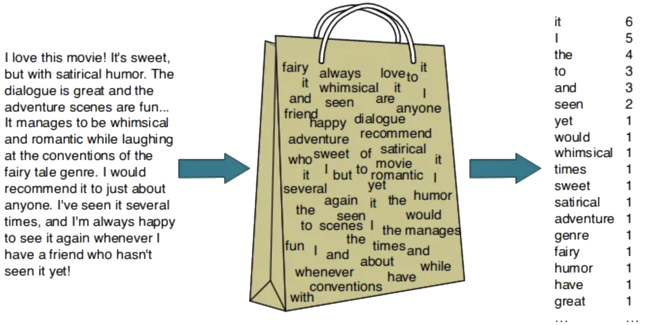
Instead, we can use Bag of Words which is an unordered dictionary of length $V$ with keys as words and values as the count of the corresponding word in the document.

Term Frequency (TF)

Term Frequency (TF) is the vector of length $V$ where each element is the count of the corresponding word in the document. It’s essentially the ordered version of Bag of Words.

Example: For the above bag of words, the term frequency vector is:

$$TF=[6,5,4,3,3,2,1,...,1,0,...,0]$$

Inverse Document Frequency (IDF)

Inverse Document Frequency (IDF) is a feature engineering technique invented in 1972 by Karen Jones. IDF gives more weight to rare words and less weight to common words across documents.

$$\text{IDF}(i)=\log \left(\frac{N}{1+D{F}_i}\right)$$

Where:

• $N$ = total number of documents
• $D{F}_i$ = number of documents containing word $i$

Example:

Word	df	idf
Romeo	1	1.57
salad	2	1.27
Falstaff	4	0.967
forest	12	0.489
battle	21	0.246
wit	34	0.037
fool	36	0.012
good	37	0
sweet	37	0

TF-IDF

Combines Term Frequency and Inverse Document Frequency to place more weight on informative words and less on uninformative ones.

$${\text{TF-IDF}}_{i,j}=\log (1+{\text{TF}}_{i,j})\times {\text{IDF}}_i$$

Where:

• ${\text{TF}}_{i,j}$ = Term Frequency of word $i$ in document $j$
• ${\text{IDF}}_i$ = Inverse Document Frequency of word $i$

Application in Search Engines

Okapi BM25 was invented by Karen Jones et al. in the 1970s. It’s a ranking function that estimates document relevance to search queries.

Given a query Q containing keywords q₁ to qₙ:

$$\text{score}(D,Q)=\sum _{i=1}^n\text{IDF}(q_i)\cdot \frac{f(q_i,D)\cdot (k_1+1)}{f(q_i,D)+k_1\cdot \left(1-b+b\cdot \frac{|D|}{\text{avgdl}}\right)}$$

Where:

• $D$ = Document
• $Q$ = Query
• $n$ = Number of keywords in the query
• $f(q_i,D)$ = Frequency of keyword $q_i$ in document $D$
• $k_1$ = Smoothing parameter
• $b$ = Length normalization parameter
• $\text{avgdl}$ = Average document length

The Word Embeddings Era

TF-IDF is a good encoding technique for search engines, but it has some limitations.

Challenges with TF-IDF:

• Curse of dimensionality: TF-IDF vector is as large as vocabulary size
• Sparsity: Many zeros in the vector
• Overfitting: With large vocabularies (e.g., 1,000,000 words) and limited training data (e.g., 1,000 examples), models overfit
• Euclidean Distance issue: Semantically similar words (like “man” and “woman”) may not be closer in vector space than dissimilar words (like “man” and “nebula”).

Solution

Word Embedding models map sparse one-hot vectors (e.g., 1,000,000 dimensions) to lower-dimensional dense vectors (e.g., 300 dimensions) where semantically similar words are placed close together.

Famous Models

• Word2Vec (2013)
• GloVe (2014) - Global Vectors for Word Representation

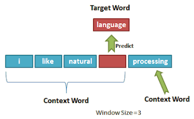
Word2Vec: Fixed Context Shallow Network

The first NLP training method using masking with two approaches:

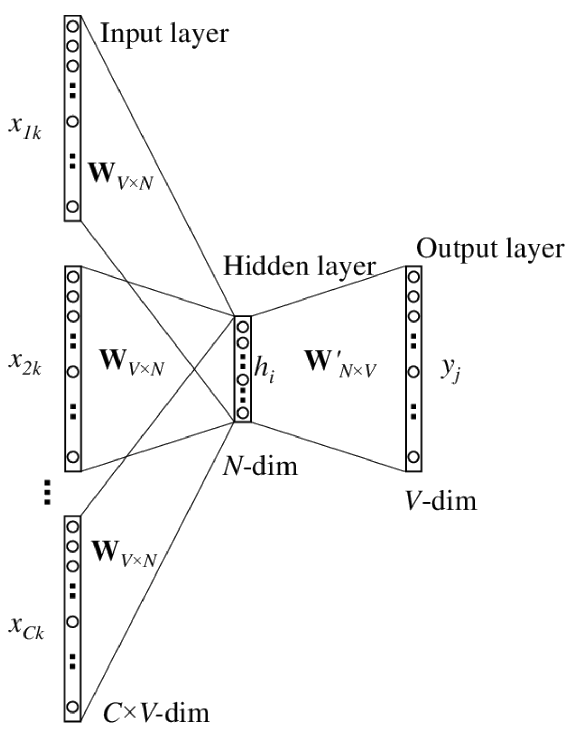
• CBOW (Continuous Bag of Words)
• Skip-gram (1 layer, context size=5)

Characteristics:

• Word embeddings are fixed during inference
• Context is not considered during inference
• Uses a shallow neural network

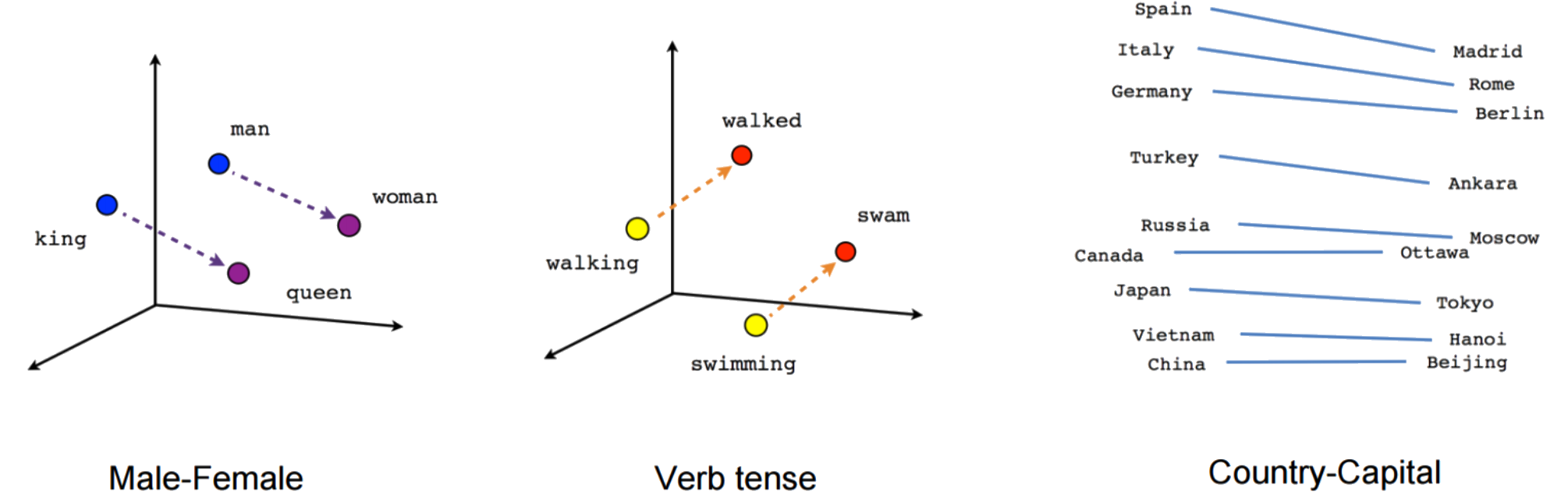
Exploring Word2Vec Embedding Space

When we reduce Word2Vec embeddings from 300 to 3 dimensions using t-SNE, we can visualize semantic relationships:

BERT: Variable Context Deep Network

BERT = Bidirectional Encoder Representations from Transformers

• Invented in 2018 at Google
• Learns adaptive word embeddings using Attention Mechanism
• Uses WordPiece tokens (30,000 tokens) instead of words
• Most famous usage of masking in NLP (Masked Language Model - MLM)
• 110 million parameters (12 layers, 12 heads, variable context)

Comparison: A Word2Vec with 400,000 words and 300-dimensional embeddings has 120 million parameters.

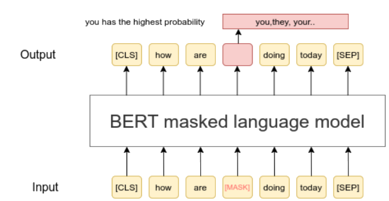
Masking in BERT Training

BERT uses masked language modeling where some tokens are randomly masked and the model learns to predict them:

From Simple-BERT to Sentence-BERT

Simple Approach: Average all word embeddings in a sentence.

Advanced Approach: Fine-tune BERT on SNLI data (Stanford Natural Language Inference) with 550,000 premise-hypothesis pairs.

Example:

• Premise: “A person on a horse jumps over a log”
• Entailing: “A person is outdoors on a horse”
• Contradicting: “A person is at a diner ordering an omelet”
• Neutral: “A person is training his horse for a competition”

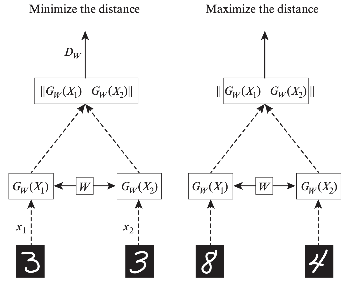
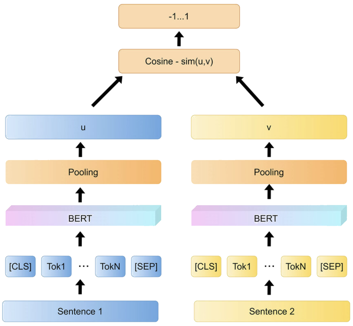
Siamese Networks & Contrastive Learning

Sentence-BERT uses siamese networks for contrastive learning:

Siamese Network for Sentence-BERT:

Siamese Network for Computer Vision: